Terminology and data models
This page describes commonly used terms used in the API and the Python client.
Curve
A Curve describes any data
series. The curve’s name is unique and identifies data series in the API.
The Curve-model contains all the meta-information which makes up its name, such
as categories, areas, unit and others.
An important attribute on the curve model is resolution (more on resolutions below). It tells you the time step (hourly, 15-minute, daily, etc.) and timezone for data in the curve.
The subscription attribute tells you what kind of subscription gives you access to the curve.
Curve types
Another essential detail is the curve_type attribute. This attribute
describes what kind of data the curve stores. There different types are:
TIMESERIESSCENARIO_TIMESERIESINSTANCEPERIODSPERIOD_INSTANCESOHLC
The curve_type tells you which operations you shall use to load data
from the curve in the API.
Subscription
A Subscription describes
your access to a curve. It contains information like the level of access,
type of subscription, a human-readable label and more information such as
the package, the area and the collection depending on the type of
subscription.
Subscription access levels
Access levels for a subscription.
FREEMIUM– Access is included in the freemium tierBLOCKED– No accessTRIAL– Access is granted during a trial periodPAYING– Access is provided through a paid subscriptionREALTO– Access is provided with a www.realto.io subscriptionINTERNAL– Access is provided through partner agreementsFREE– Access is available at no costNONE– Missing access information
Subscription types
The type of subscription.
COLLECTION– A subscription related to collectionsFREE– No subscription required for provided contentFREEMIUM– Limited access due to no subscription defined for provided contentPACKAGE– A subscription associated with a package of servicesPACKAGE_AREA– A subscription tied to a combination of a specific package and areaPRIVATE– A private subscription with restricted access
Subscription collection permissions
The user’s permissions for a collection.
r– Read-only accessrw– Read-write access
Instance
Some data series, such as those that contain forecasts, are not only one series, but a collection of many series. We call each of these series instances.
An Instance is identified by
the combination of two attributes: An issue date (date-time) and a tag
(string).
For instance, Energy Quantified’s forecasts based on the weather
forecast ECMWF uses tag = 'ec' and the
issue date as specified by ECMWF. So the morning forecast has these
attributes:
# ECMWF deterministic forecast at midnight on 1 January 2020
instance.issued = datetime(2020, 1, 1, 0, 0, 0, 0, tz=UTC)
instance.tag = 'ec'
Time series that are instances (forecasts) have an instance attribute.
Place
The Place model is a rather
generic: It represents anything that has a geographical location, and
therefore it has a latitude and longitude.
Places have a type attribute describing what you may find in this
place! These types are currently:
producer– Powerplant. Where available, you will also get afuelattribute with the production type (wind, solar, nuclear, etc.).consumer– Factory or otherwise large consumer of powerweatherstation– A weather stationriver– A point on a river (used for river temperature forecasts at critical locations)
Curves may be linked to a place (for instance actual production for a nuclear power plant). And a place has a list of all curves connected to it.
Resolution, timezone and frequency
Power markets operate on contracts such as 15-minute, hourly, daily, weekly, monthly, quarterly and yearly. We call these different time intervals for frequencies.
Frequency
A frequency is a time step. We use mostly ISO-8601-style naming of frequencies, but with a few exceptions. See Duration (Wikipedia) for an excellent explanation of the format.
P1Y– YearlySEASON– Summer or winterP3M– QuarterlyP1M– MonthlyP1W– WeeklyP1D– DailyPT1H– HourlyPT30M– 30 minutesPT15M– 15 minutesPT10M– 10 minutesPT5M– 5 minutes
The SEASON frequency is used for gas market contracts. It starts on 1
April (summer) or 1 October (winter) and lasts six months.
Besides, the following frequency constant is used when data does not follow a fixed interval (such as tick data). It is an invalid frequency for operations that involve the Timeseries model.
NONE– No frequency specified (i.e. tick data)
See the Frequency enum class
for more details.
Timezone
These are the most commonly used timezones. Most power markets in Europe operate in CET due to standardization and market coupling.
UTC– Coordinated Universal TimeWET– Western European TimeCET– Central European TimeEET– Eastern European TimeEurope/Istanbul– Turkey TimeEurope/Moscow– Russian/Moscow TimeEurope/Gas_Day– (Non-standard timezone; not in the IANA timezone database) European Gas Day at UTC-0500 (UTC-0400 during Daylight Saving Time). Starts at 06:00 in CE(S)T time. Used for the natural gas market in the European Union.
We use the pytz library for timezones.
Resolution
It is a combination of a frequency and a timezone. All time series have a
resolution. Only resolutions with iterable frequencies are iterable (meaning
all frequencies other than NONE).
With Energy Quantified’s Python library, you can do something like this:
>>> from energyquantified.time import (
>>>    Resolution, Frequency, UTC, get_datetime
>>> )
>>> resolution = Resolution(Frequency.P1D, UTC)
>>> begin = get_datetime(2020, 1, 1, tz=UTC)
>>> end = get_datetime(2020, 1, 5, tz=UTC)
>>> for d in resolution.enumerate(begin, end):
>>>     print(d)
2020-01-01 00:00:00+00:00
2020-01-02 00:00:00+00:00
2020-01-03 00:00:00+00:00
2020-01-04 00:00:00+00:00
Of course, you could use datetime.timedelta from the standard Python
library to achieve a similar result. However, datetime.timedelta does not
handle the transition from/to daylight saving time. Using the Resolution
will make sure that the date-times get the right offset from UTC.
See the Resolution class for
a full reference.
Aggregation and filters
Aggregation
To aggregate means to downsample data to a lower resolution. Example: Convert hourly values to daily values.
When aggregating, you must choose a strategy for how to calculate the aggregated value. The supported aggregations are:
AVERAGE– The mean of all input values
SUM– Sum of all input values
MIN– Find the lowest value
MAX– Find the highest value
Energy Quantified defaults to use AVERAGE (mean).
Class reference: Aggregation
Filters (or hour-filters)
You can also apply filters on which hours you want to include in aggregations.
In the power markets, one typically make a distinction between base and peak hours. Some weekly contracts traditionally also separate workdays from weekends. Here are some explanations:
BASE– All hoursPEAK– Peak hours (8-20). For future contracts: Peak hours (8-20) during workdaysOFFPEAK– Offpeak (0-8 and 20-24). For future contracts: Offpeak hours (0-8 and 20-24) during workdays and all hours during the weekendWORKDAYS– Monday, Tuesday, Wednesday, Thursday, FridayWEEKENDS– Saturday, Sunday
Important: When loading aggregated time series data from the API, you should keep the following in mind:
For weekly, monthly, quarterly and yearly resolutions,
PEAKis defined asPEAKhours duringWORKDAYS(8-20 during workdays).OFFPEAKis, for the same resolutions, defined asOFFPEAKhours duringWORKDAYSand all hours duringWEEKENDS.For daily resolutions,
PEAKandOFFPEAKdo not make a distinction between workdays and weekends.
Class reference: Filter
Conversions
Unit
Convert data to another unit. Supported units at this moment:
°Cfor temperatures in celsius degreesDegreesfor angles in degreeshPafor pressure in hectopascalmfor length in metersm^2for area in square metersm^3for volume in cubic meterssfor time in secondstfor weight in tonsTW,GW,MW,kW,Wfor power in wattTWh,GWh,MWh,kWh,Whfor energy in watt-hoursTWh/h,GWh/h,MWh/h,kWh/h,Wh/hfor average energy in watt-hours per hourthermfor heat energy in thermsbblfor volume in barrels%as percentEUR,USD,GBP,NOK,SEK,DKK,CHF,CZK,HUF,PLN,BGN,HRK,RUB,RON,TRY,pencefor currencies
Note: Currency conversions are not supported for timeseries with a frequency higher than P1D and not for periods.
Aggregation threshold
By default, the aggregation returns empty values whenever one or more input values are missing. You can set a threshold that defines how many values are allowed to be missing within a frame of the converted frequency. If the number of missing values is less than or equal to the threshold, aggregation is performed on the remaining non-empty values. Otherwise, an empty value is returned.
Note: By default, the threshold is set to zero. This means that an empty input value will result in an empty output value.
For example, you want to convert hourly values to daily values using the mean value. Let’s assume that some input values are missing. Instead of getting empty values, you want to get the average if a maximum of four values are missing within a day. In this case, set the threshold to four.
Time series
A Timeseries is a data series
with date-times as the index. Time series in Energy Quantified’s API has a
fixed interval (i.e. 15-minute, hourly, daily). For time series with
varying duration per item, see [Period series](#period-series).
Example of a time series:
Date         Value
----------  ------
2020-01-01   145.2
2020-01-02   156.9
2020-01-03   167.4
2020-01-04   134.1
...
Time series data can have a varying number of values per date-time:
Single-value: Each
date-timehas one corresponding value.Scenarios: Each
date-timehas multiple values.Scenarios with mean value: Each
date-timehas multiple values and a mean value of those scenarios.
Scenarios are sometimes also referred to as ensembles. This terminology comes from meteorology, where forecasts with multiple scenarios are called ensemble forecasts. For instance, the ECMWF ensemble forecast has 51 scenarios, and the GFS ensemble forecast has 21 scenarios.
Period series
While Time series’ are excellent for representing fixed-interval data, some time series data can be stored and served more efficient.
For instance, there are plenty of capacity plans published in the power markets (i.e. REMIT). Another example is assumptions on installed capacity on different fuel types in the future. Such data often have the same value over an extended period, and the value changes sporadically.
So Energy Quantified created what we call a
Periodseries for this, which
is a collection of date-time ranges with a begin date-time, an end
date-time, and a corresponding value.
The client also supports converting any such period series to a time series in your preferred resolution.
Example of a period series:
Begin       End          Value
----------  ----------  ------
2020-01-01  2020-01-05     300    #  4 days
2020-01-05  2020-02-01     125    # 27 days
2020-02-01  2020-02-13     160    # 12 days
2020-02-13  2020-02-14     220    #  1 day
...
Period-based series has two different types of periods:
Period with a value: Each period has one corresponding value, like in the example table above.
Period with a value and a capacity: Each period has a current value and a total installed capacity. These types of values appear mostly in REMIT data, where the value is the currently available production capacity, while the total installed capacity is provided for reference.
OHLC
End-of-day statistics for financial contracts. OHLC stands for open, high, low and close, and is a summary of trades for a day. OHLC is typically used to illustrate movements in the price of a financial instrument and can be seen in financial charts looking like candlesticks.
In cooperation Montel, Energy Quantified
provides OHLC data for all power
market regions in Europe, as well as prices for gas markets, carbon emissions
(EUA), brent oil and coal (API2).
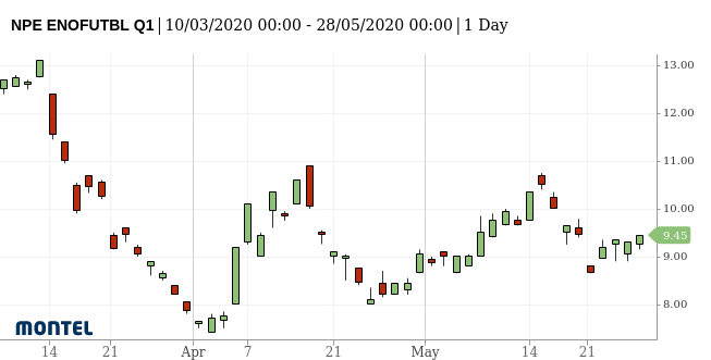
Example: The Nasdaq Nordic Power Future contract for a front quarter contract (Q1).
SRMC
In the power market, the short-run marginal cost of running power plants. See short-run marginal cost on Wikipedia for a broader definition.
Energy Quantified allows SRMC calculations for gas- and coal-fired power production.
Next steps
Learn how to connect to the API and to discover data.
