Quickstart
This page gives a short introduction on how to get started with Energy Quantified’s Python library.
2-minute guide
First, make sure that energyquantified is installed and up-to-date
on your workstation.
Authenticate
Import the library, create a client and supply the API key:
>>> from energyquantified import EnergyQuantified
>>> eq = EnergyQuantified(api_key='aaaa-bbbb-cccc-dddd')
You can check if your API key is valid by invoking is_api_key_valid():
>>> eq.is_api_key_valid()
True
Search for curves (data series)
Energy Quantified allows you to search for curves in two ways. By free-text search:
>>> curves = eq.metadata.curves(q='wind power germany actual')
>>> curves
[<Curve: "DE Wind Power Production MWh/h 15min Actual", curve_type=TIMESERIES, subscription=FREEMIUM>,
 <Curve: "DE Wind Power Production Offshore MWh/h 15min Actual", curve_type=TIMESERIES, subscription=FREEMIUM>,
 <Curve: "DE Wind Power Production Onshore MWh/h 15min Actual", curve_type=TIMESERIES, subscription=FREEMIUM>,
 <Curve: "DE-50Hertz Wind Power Production MWh/h 15min Actual", curve_type=TIMESERIES, subscription=FREEMIUM>,
 <Curve: "DE-Amprion Wind Power Production MWh/h 15min Actual", curve_type=TIMESERIES, subscription=FREEMIUM>,
 ...
Or by filtering on specific terms:
>>> curves = eq.metadata.curves(area='de', data_type='actual', category=['Wind', 'Power'])
>>> curves
[<Curve: "DE Wind Power Production MWh/h 15min Actual", curve_type=TIMESERIES, subscription=FREEMIUM>,
 <Curve: "DE Wind Power Production Offshore MWh/h 15min Actual", curve_type=TIMESERIES, subscription=FREEMIUM>,
 <Curve: "DE Wind Power Production Onshore MWh/h 15min Actual", curve_type=TIMESERIES, subscription=FREEMIUM>]
Load data
When you have found your curve, you can download it. As these curves are of
curve_type = TIMESERIES, we should use the eq.timeseries.load()-function.
When specifying the curve parameter in the load()-function, you can
either provide a Curve instance and a string. Same for the dates (either
provide a Python date, datetime, or an ISO-8601-like string YYYY-MM-DD).
>>> from datetime import date
>>> timeseries = eq.timeseries.load(
>>>    'DE Wind Power Production MWh/h 15min Actual',
>>>    begin=date(2020, 1, 1),
>>>    end=date(2020, 2, 1)
>>> )
The result will be a Timeseries with all the attributes parsed into Python-objects.
>>> timeseries.curve
<Curve: "DE Wind Power Production MWh/h 15min Actual", curve_type=TIMESERIES, subscription=FREEMIUM>
>>> timeseries.resolution
<Resolution: frequency=PT15M, timezone=CET>
>>> timeseries.data[:4]
[<Value: date=2020-01-01 00:00:00+01:00, value=6387>,
 <Value: date=2020-01-01 00:15:00+01:00, value=6383>,
 <Value: date=2020-01-01 00:30:00+01:00, value=6640>,
 <Value: date=2020-01-01 00:45:00+01:00, value=6882>]
You can also loop over the values in a Timeseries like this:
>>> for v in timeseries:
>>>     print(v)
<Value: date=2020-01-01 00:00:00+01:00, value=6387>
<Value: date=2020-01-01 00:15:00+01:00, value=6383>
<Value: date=2020-01-01 00:30:00+01:00, value=6640>
...
Now it’s up to you to decide the next step. You could save the data to your own database, or perhaps start doing some data analysis.
Use pandas for data analysis
(You need to install pandas separately to do this.) Convert any time series
to a pandas.DataFrame like so:
>>> df = timeseries.to_pandas_dataframe(name='series')
>>> df
                           series


date
2020-01-01 00:00:00+01:00    6387
2020-01-01 00:15:00+01:00    6383
2020-01-01 00:30:00+01:00    6640
2020-01-01 00:45:00+01:00    6882
...                           ...
Use polars for data analysis
(You need to install polars separately to do this.) Convert any time series
to a polars.DataFrame like so:
>>> df = timeseries.to_polars_dataframe(name='series')
>>> df
shape: (96, 2)
┌─────────────────────────┬─────────┐
│ date                    ┆ series  │
│ ---                     ┆ ---     │
│ datetime[μs, CET]       ┆ f64     │
╞═════════════════════════╪═════════╡
│ 2020-01-01 00:00:00 CET ┆ 6405.0  │
│ 2020-01-01 00:15:00 CET ┆ 6388.0  │
│ 2020-01-01 00:30:00 CET ┆ 6650.0  │
│ 2020-01-01 00:45:00 CET ┆ 6893.0  │
│ 2020-01-01 01:00:00 CET ┆ 6975.0  │
│ …                       ┆ …       │
│ 2020-01-01 22:45:00 CET ┆ 12414.0 │
│ 2020-01-01 23:00:00 CET ┆ 12382.0 │
│ 2020-01-01 23:15:00 CET ┆ 12528.0 │
│ 2020-01-01 23:30:00 CET ┆ 12390.0 │
│ 2020-01-01 23:45:00 CET ┆ 12392.0 │
└─────────────────────────┴─────────┘
Mini-guide to pandas and matplotlib
Before you continue: You need to install pandas and matplotlib to
follow this mini-guide.
Load some data:
First, let’s import all we need and load the data:
>>> # Find curves
>>> curve_wind = eq.metadata.curves(q="de wind prod actual")[0]
>>> curve_solar = eq.metadata.curves(q="de solar photovoltaic prod actual")[0]
>>> curve_wind, curve_solar
(<Curve: "DE Wind Power Production MWh/h 15min Actual", curve_type=TIMESERIES, subscription=FREEMIUM>,
 <Curve: "DE Solar Photovoltaic Production MWh/h 15min Actual", curve_type=TIMESERIES, subscription=FREEMIUM>)

>>> # Load data
>>> wind = eq.timeseries.load(curve_wind, begin='2020-03-25', end='2020-04-01')
>>> solar = eq.timeseries.load(curve_solar, begin='2020-03-25', end='2020-04-01')
Using pandas:
Convert to both the wind and solar time series to pandas.DataFrame instances
like so:
>>> import pandas as pd
>>> import matplotlib.pyplot as plt

>>> df_solar = solar.to_pandas_dataframe(name='de solar')
>>> df_wind = wind.to_pandas_dataframe(name='de wind')
>>> df_wind
                           de wind


date
2020-03-25 00:00:00+01:00    25049
2020-03-25 00:15:00+01:00    24810
2020-03-25 00:30:00+01:00    24648
2020-03-25 00:45:00+01:00    24395
2020-03-25 01:00:00+01:00    23992
...                            ...
2020-03-31 22:45:00+02:00     9919
2020-03-31 23:00:00+02:00    10098
2020-03-31 23:15:00+02:00    10318
2020-03-31 23:30:00+02:00    10563
2020-03-31 23:45:00+02:00    10556

[668 rows x 1 columns]
You can then concatenate these two into one DataFrame.
Supplying axis=1 means that you concatenate columns, which in this case
add the columns next to each other while maintaining the dates. (Using
axis=0 will concatenate on the index, which in this case are the dates.
That will yield an unwanted result.)
>>> df = pd.concat([dfw, dfs], axis=1)
>>> df
                           de wind  de solar


date
2020-03-25 00:00:00+01:00    25049         0
2020-03-25 00:15:00+01:00    24810         0
2020-03-25 00:30:00+01:00    24648         0
2020-03-25 00:45:00+01:00    24395         0
2020-03-25 01:00:00+01:00    23992         0
...                            ...       ...
2020-03-31 22:45:00+02:00     9919         0
2020-03-31 23:00:00+02:00    10098         0
2020-03-31 23:15:00+02:00    10318         0
2020-03-31 23:30:00+02:00    10563         0
2020-03-31 23:45:00+02:00    10556         0

[668 rows x 2 columns]
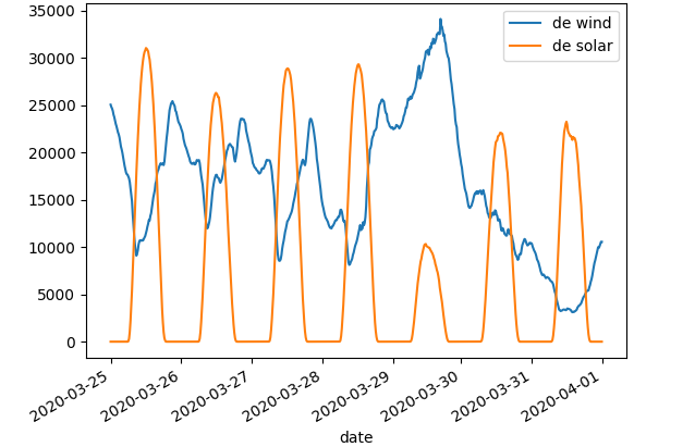
Below is an example where we plot the data and export it to a file in the
current working directory called 15min_chart.png. It uses the original
DataFrame with 15-minute resolution data.
>>> # Plot and save to file
>>> df.plot()
>>> plt.savefig('15min_chart.png')
You can also perform aggregations:
>>> # Use pandas to aggregate to daily mean production
>>> df2 = df.resample('D').mean()
>>> df2
                                de wind     de solar


date
2020-03-25 00:00:00+01:00  18112.416667  9349.697917
2020-03-26 00:00:00+01:00  18977.197917  7868.750000
2020-03-27 00:00:00+01:00  16811.010417  8655.989583
2020-03-28 00:00:00+01:00  15940.093750  8773.229167
2020-03-29 00:00:00+01:00  27446.750000  3451.119565
2020-03-30 00:00:00+02:00  12960.114583  6863.718750
2020-03-31 00:00:00+02:00   5968.635417  7462.677083
And you can add the wind and solar production together to create a sum
of renewables. The result will be a pandas.Series, as indicated by the
Freq: D in the bottom.
>>> df2['de wind'] + df2['de solar']
date
2020-03-25 00:00:00+01:00    27462.114583
2020-03-26 00:00:00+01:00    26845.947917
2020-03-27 00:00:00+01:00    25467.000000
2020-03-28 00:00:00+01:00    24713.322917
2020-03-29 00:00:00+01:00    30897.869565
2020-03-30 00:00:00+02:00    19823.833333
2020-03-31 00:00:00+02:00    13431.312500
Freq: D, dtype: float64
Find out more about pandas and matplotlib:
Look at the pandas and matplotlib documentation for a more in-depth explanation of concepts and features.
Mini-guide to polars
Before you continue: You need to install polars follow this mini-guide.
Load some data:
First, let’s import all we need and load the data:
>>> # Find curves
>>> curve_wind = eq.metadata.curves(q="de wind prod actual")[0]
>>> curve_solar = eq.metadata.curves(q="de solar photovoltaic prod actual")[0]
>>> curve_wind, curve_solar
(<Curve: "DE Wind Power Production MWh/h 15min Actual", curve_type=TIMESERIES, subscription=FREEMIUM>,
 <Curve: "DE Solar Photovoltaic Production MWh/h 15min Actual", curve_type=TIMESERIES, subscription=FREEMIUM>)

>>> # Load data
>>> wind = eq.timeseries.load(curve_wind, begin='2020-03-25', end='2020-04-01')
>>> solar = eq.timeseries.load(curve_solar, begin='2020-03-25', end='2020-04-01')
Using polars:
Convert to both the wind and solar time series to polars.DataFrame instances
like so:
>>> import polars as pl
>>> df_solar = solar.to_polars_dataframe(name='de solar')
>>> df_wind = wind.to_polars_dataframe(name='de wind')
>>> df_wind
shape: (668, 2)
┌──────────────────────────┬─────────┐
│ date                     ┆ de wind │
│ ---                      ┆ ---     │
│ datetime[μs, CET]        ┆ f64     │
╞══════════════════════════╪═════════╡
│ 2020-03-25 00:00:00 CET  ┆ 24945.0 │
│ 2020-03-25 00:15:00 CET  ┆ 24764.0 │
│ 2020-03-25 00:30:00 CET  ┆ 24631.0 │
│ 2020-03-25 00:45:00 CET  ┆ 24313.0 │
│ 2020-03-25 01:00:00 CET  ┆ 23903.0 │
│ …                        ┆ …       │
│ 2020-03-31 22:45:00 CEST ┆ 10000.0 │
│ 2020-03-31 23:00:00 CEST ┆ 10161.0 │
│ 2020-03-31 23:15:00 CEST ┆ 10397.0 │
│ 2020-03-31 23:30:00 CEST ┆ 10636.0 │
│ 2020-03-31 23:45:00 CEST ┆ 10614.0 │
└──────────────────────────┴─────────┘
You can then concatenate these two into one DataFrame.
Supplying how="align" combines frames horizontally, auto-determining the
common key columns and aligning rows using the same logic as (if you need more
control over this you should use a suitable join method directly)
>>> df = pl.concat([df_wind, df_solar], how="align")
>>> df
shape: (668, 3)
┌──────────────────────────┬─────────┬──────────┐
│ date                     ┆ de wind ┆ de solar │
│ ---                      ┆ ---     ┆ ---      │
│ datetime[μs, CET]        ┆ f64     ┆ f64      │
╞══════════════════════════╪═════════╪══════════╡
│ 2020-03-25 00:00:00 CET  ┆ 24945.0 ┆ 0.0      │
│ 2020-03-25 00:15:00 CET  ┆ 24764.0 ┆ 0.0      │
│ 2020-03-25 00:30:00 CET  ┆ 24631.0 ┆ 0.0      │
│ 2020-03-25 00:45:00 CET  ┆ 24313.0 ┆ 0.0      │
│ 2020-03-25 01:00:00 CET  ┆ 23903.0 ┆ 0.0      │
│ …                        ┆ …       ┆ …        │
│ 2020-03-31 22:45:00 CEST ┆ 10000.0 ┆ 0.0      │
│ 2020-03-31 23:00:00 CEST ┆ 10161.0 ┆ 0.0      │
│ 2020-03-31 23:15:00 CEST ┆ 10397.0 ┆ 0.0      │
│ 2020-03-31 23:30:00 CEST ┆ 10636.0 ┆ 0.0      │
│ 2020-03-31 23:45:00 CEST ┆ 10614.0 ┆ 0.0      │
└──────────────────────────┴─────────┴──────────┘
>>> df = df_wind.join(df_solar, how="full", on="date", coalesce=True)
>>> df
shape: (668, 3)
┌──────────────────────────┬─────────┬──────────┐
│ date                     ┆ de wind ┆ de solar │
│ ---                      ┆ ---     ┆ ---      │
│ datetime[μs, CET]        ┆ f64     ┆ f64      │
╞══════════════════════════╪═════════╪══════════╡
│ 2020-03-25 00:00:00 CET  ┆ 24945.0 ┆ 0.0      │
│ 2020-03-25 00:15:00 CET  ┆ 24764.0 ┆ 0.0      │
│ 2020-03-25 00:30:00 CET  ┆ 24631.0 ┆ 0.0      │
│ 2020-03-25 00:45:00 CET  ┆ 24313.0 ┆ 0.0      │
│ 2020-03-25 01:00:00 CET  ┆ 23903.0 ┆ 0.0      │
│ …                        ┆ …       ┆ …        │
│ 2020-03-31 22:45:00 CEST ┆ 10000.0 ┆ 0.0      │
│ 2020-03-31 23:00:00 CEST ┆ 10161.0 ┆ 0.0      │
│ 2020-03-31 23:15:00 CEST ┆ 10397.0 ┆ 0.0      │
│ 2020-03-31 23:30:00 CEST ┆ 10636.0 ┆ 0.0      │
│ 2020-03-31 23:45:00 CEST ┆ 10614.0 ┆ 0.0      │
└──────────────────────────┴─────────┴──────────┘
You can also perform aggregations:
>>> import polars.selectors as cs
>>> # Use polars to aggregate to daily mean production
>>> df2 = df.group_by_dynamic("date", every="1d").agg(cs.exclude("date").mean())
>>> df2
shape: (7, 3)
┌──────────────────────────┬──────────────┬─────────────┐
│ date                     ┆ de wind      ┆ de solar    │
│ ---                      ┆ ---          ┆ ---         │
│ datetime[μs, CET]        ┆ f64          ┆ f64         │
╞══════════════════════════╪══════════════╪═════════════╡
│ 2020-03-25 00:00:00 CET  ┆ 18104.34375  ┆ 9349.697917 │
│ 2020-03-26 00:00:00 CET  ┆ 19041.583333 ┆ 7868.75     │
│ 2020-03-27 00:00:00 CET  ┆ 16855.78125  ┆ 8655.989583 │
│ 2020-03-28 00:00:00 CET  ┆ 15982.739583 ┆ 8773.229167 │
│ 2020-03-29 00:00:00 CET  ┆ 27489.141304 ┆ 3451.119565 │
│ 2020-03-30 00:00:00 CEST ┆ 12937.989583 ┆ 6863.71875  │
│ 2020-03-31 00:00:00 CEST ┆ 5945.114583  ┆ 7462.677083 │
└──────────────────────────┴──────────────┴─────────────┘
And you can add the wind and solar production together to create a sum of renewables.
>>> df3 = df2.with_columns(pl.col('de wind').add(pl.col('de solar')).alias('de renewables'))
>>> df3
shape: (7, 4)
┌──────────────────────────┬──────────────┬─────────────┬───────────────┐
│ date                     ┆ de wind      ┆ de solar    ┆ de renewables │
│ ---                      ┆ ---          ┆ ---         ┆ ---           │
│ datetime[μs, CET]        ┆ f64          ┆ f64         ┆ f64           │
╞══════════════════════════╪══════════════╪═════════════╪═══════════════╡
│ 2020-03-25 00:00:00 CET  ┆ 18104.34375  ┆ 9349.697917 ┆ 27454.041667  │
│ 2020-03-26 00:00:00 CET  ┆ 19041.583333 ┆ 7868.75     ┆ 26910.333333  │
│ 2020-03-27 00:00:00 CET  ┆ 16855.78125  ┆ 8655.989583 ┆ 25511.770833  │
│ 2020-03-28 00:00:00 CET  ┆ 15982.739583 ┆ 8773.229167 ┆ 24755.96875   │
│ 2020-03-29 00:00:00 CET  ┆ 27489.141304 ┆ 3451.119565 ┆ 30940.26087   │
│ 2020-03-30 00:00:00 CEST ┆ 12937.989583 ┆ 6863.71875  ┆ 19801.708333  │
│ 2020-03-31 00:00:00 CEST ┆ 5945.114583  ┆ 7462.677083 ┆ 13407.791667  │
└──────────────────────────┴──────────────┴─────────────┴───────────────┘
Find out more about polars:
Look at the polars a documentation for a more in-depth explanation of concepts and features.
Next steps
Get familiar with terminology and data types used in the Energy Quantified API and in the Energy Quantified Python library:
