Terminology and data models
This page describes commonly used terms used in the API and the Python client.
Curve
A curve describes any time series data. The curve’s name is unique and identifies data series in the API. The Curve-model contains all the meta-information which makes up its name, such as categories, areas, unit and others.
A curve has a resolution (see below).
Curve types
Another essential detail is the curve_type attribute. This attribute
describes what kind of data the curve stores. There different types are:
TIMESERIESSCENARIO_TIMESERIESINSTANCEPERIODSPERIOD_INSTANCESOHLC
Instance
Some data series, such as those that contain forecasts, are not only one series, but a collection of many series. We call each of these series instances.
The instances are identified by the combination of two attributes: An issue date (date-time) and a tag (string).
For instance, Energy Quantified’s forecasts based on the weather
forecast ECMWF uses tag = 'ec' and the
issue date as specified by ECMWF. So the morning forecast has these
attributes:
# ECMWF deterministic forecast at midnight on 1 January 2020
instance.issued = datetime(2020, 1, 1, 0, 0, 0, 0, tz=UTC)
instance.tag = 'ec'
Time series that are instances have an instance attribute.
Place
The Place model is a rather generic: It represents anything that has a geographical location, and therefore it has a latitude and longitude.
Places have a type attribute describing what you may find in this
place! These types are currently:
producer– Powerplant. Where available, you will also get afuelattribute with the production type (wind, solar, nuclear, etc.).consumer– Factory or otherwise large consumer of powerweatherstation– A weather stationriver– A point on a river (used for river temperature forecasts at critical locations)
Curves may be linked to a place (for instance actual production for a nuclear power plant). And a place has a list of all curves connected to it.
Resolution, time-zone and frequency
Power markets operate on contracts such as 15-minute, hourly, daily, weekly, monthly, quarterly and yearly. We call these different time intervals for frequencies.
Frequency
A frequency is a time step. We use mostly ISO-8601-style naming of frequencies, but with a few exceptions. See Duration (Wikipedia) for an excellent explanation of the format.
P1Y– YearlySEASON– Summer or winterP3M– QuarterlyP1M– MonthlyP1W– WeeklyP1D– DailyPT1H– HourlyPT30M– 30 minutesPT15M– 15 minutesPT10M– 10 minutesPT5M– 5 minutes
The SEASON frequency is used for gas market contracts. It starts on 1
April (summer) or 1 October (winter) and lasts six months.
Besides, the following frequency constant is used when data does not follow a fixed interval (such as tick data). It is an invalid frequency for operations that involve the Timeseries model.
NONE– No frequency specified (i.e. tick data)
See the Frequency enum class for more details.
Time-zone
These are the most commonly used time-zones. Most power markets in Europe operate in CET due to standardization and market coupling.
UTC– Coordinated Universal TimeWET– Western European TimeCET– Central European TimeEET– Eastern European TimeEurope/Istanbul– Turkey TimeEurope/Moscow– Russian/Moscow TimeEurope/Gas_Day– (Non-standard time-zone; not in the IANA time-zone database) European Gas Day at UTC-0500 (UTC-0400 during Daylight Saving Time). Starts at 06:00 in CE(S)T time. Used for the natural gas market in the European Union.
We use the pytz library for time-zones.
Resolution
It is a combination of a frequency and a time-zone. All time series have a
resolution. Only resolutions with iterable frequencies are iterable (meaning
all frequencies other than NONE).
With Energy Quantified’s Python library, you can do something like this:
>>> from energyquantified.time import (
>>>    Resolution, Frequency, UTC, get_datetime
>>> )
>>> resolution = Resolution(Frequency.P1D, UTC)
>>> begin = get_datetime(2020, 1, 1, tz=UTC)
>>> end = get_datetime(2020, 1, 5, tz=UTC)
>>> for d in resolution.enumerate(begin, end):
>>>     print(d)
2020-01-01 00:00:00+00:00
2020-01-02 00:00:00+00:00
2020-01-03 00:00:00+00:00
2020-01-04 00:00:00+00:00
Of course, you could use datetime.timedelta from the standard Python
library to achieve a similar result. However, timedelta does not handle
the transition from/to daylight saving time, so using the Resolution will
make sure that the date-times get the right offset from UTC.
See the Resolution class for more information.
Aggregation and filters
Aggregation
To aggregate means to downsample data to a lower resolution. Example: Convert hourly values to daily values.
When aggregating, you must choose a strategy for how to calculate the aggregated value. The supported aggregations are:
AVERAGE– The mean of all input valuesSUM– Sum of all input valuesMIN– Find the lowest valueMAX– Find the highest value
Energy Quantified defaults to use AVERAGE (mean).
The aggregation will return empty values whenever there are one or more missing input values.
Filters (or hour-filters)
You can also apply filters on which hours you want to include in aggregations.
In the power markets, one typically make a distinction between base and peak hours. Some weekly contracts traditionally also separate workdays from weekends. Here are some explanations:
BASE– All hoursPEAK– Peak hours (8-20). For future contracts: Peak hours (8-20) during workdaysOFFPEAK– Offpeak (0-8 and 20-24). For future contracts: Offpeak hours (0-8 and 20-24) during workdays and all hours during the weekendWORKDAYS– Monday, Tuesday, Wednesday, Thursday, FridayWEEKENDS– Saturday, Sunday
Important: When loading aggregated time series data from the API, you should keep the following in mind:
For weekly, monthly, quarterly and yearly resolutions,
PEAKis defined asPEAKhours duringWORKDAYS(8-20 during workdays).OFFPEAKis, for the same resolutions, defined asOFFPEAKhours duringWORKDAYSand all hours duringWEEKENDS.For daily resolutions,
PEAKandOFFPEAKdo not make a distinction between workdays and weekends.
Time series
A time series is a data series with date-times as the index. Time series in Energy Quantified’s API has a fixed interval (i.e. 15-minute, hourly, daily). For time series with varying duration per item, see Period series.
Example of a time series:
Date         Value
----------  ------
2020-01-01   145.2
2020-01-02   156.9
2020-01-03   167.4
2020-01-04   134.1
...
Time series data can have a varying number of values per date-time:
Single-value: Each
date-timehas one corresponding value.Scenarios: Each
date-timehas multiple values.Scenarios with mean value: Each
date-timehas multiple values and a mean value of those scenarios.
Scenarios are sometimes also referred to as ensembles. This terminology comes from meteorology, where forecasts with multiple scenarios are called ensembles. For instance, the ECMWF ensemble forecast has 51 scenarios, and the GFS ensemble forecast has 21 scenarios.
Period series
While the Time series class is excellent for representing fixed-interval data, some time series data can be stored and served more efficient.
For instance, there are plenty of capacity plans published in the power markets (i.e. REMIT). Another example is assumptions on installed capacity on different fuel types in the future. Such data often have the same value over an extended period, and the value changes sporadically.
So Energy Quantified created what we call a period series for this, which is a collection of date-time ranges with a begin date-time, an end date-time, and a corresponding value.
The Energy Quantified Python client also supports converting any such period series to a time series in your preferred resolution.
Example of a period series:
Begin       End          Value
----------  ----------  ------
2020-01-01  2020-01-05     300    (4 days)
2020-01-05  2020-02-01     125   (27 days)
2020-02-01  2020-02-13     160   (12 days)
2020-02-13  2020-02-14     220    (1 day)
...
Period-based series has two different types of periods:
Period with a value: Each period has one corresponding value, like in the example table above.
Period with a value and a capacity: Each period has a current value and a total installed capacity. These types of values appear mostly in REMIT data, where the value is the currently available production capacity, while the total installed capacity is provided for reference.
OHLC
End-of-day statistics for financial contracts. OHLC stands for open, high, low and close, and is a summary of trades for a day. OHLC is typically used to illustrate movements in the price of a financial instrument and can be seen in financial charts looking like candlesticks.
In cooperation Montel, Energy Quantified provides OHLC data for all power market regions in Europe, as well as prices for gas markets, carbon emissions (EUA), brent oil and coal (API2).
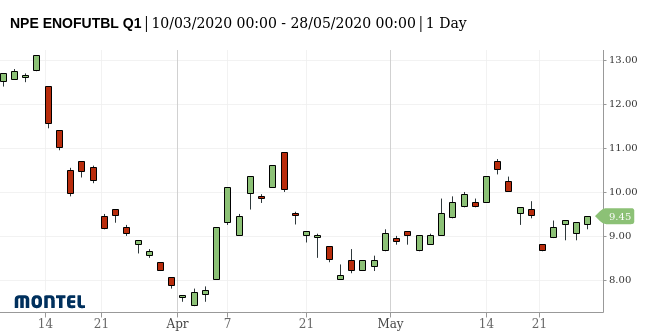
Example: Nord Pool future contract for a front quarter contract (Q1).
SRMC, dark- and spark spreads
SRMC
In the power market, the short-run marginal cost of running power plants. See short-run marginal cost on Wikipedia for a broader definition.
Dark- and spark spreads
See the section on clean spreads on Wikipedia.
Next steps
Learn how to connect to the API and to discover data.
